
If you're looking for ways to make your spreadsheet stand out, Microsoft Excel 2013 gives you an option you may not have thought to look for: the Gridline Color setting. This setting, which you can find after a few clicks in a worksheet's File Options, lets you change the gridlines around the cells from the default gray to any of 56 different colors. If you use borders around the cells, Excel gives you even more color options.
Changing the Gridline Color
Video of the Day
Step 1
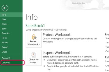
Open an Excel workbook and select the worksheet you want to change. Click the "File" menu and select "Options."
Video of the Day
Step 2
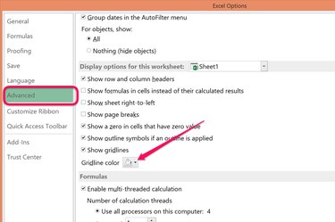
Click "Advanced" and scroll down to the Display Options for this Worksheet section. Make sure the Show Gridlines box is checked, which is the default setting. Click the "Gridline Color" menu.
Step 3
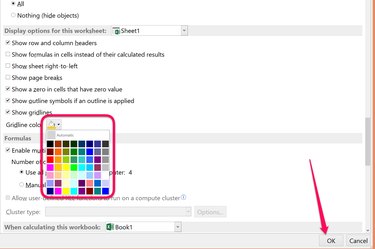
Select any color from the Gridline Color palette, then click "OK." The gridlines surrounding the cells in your worksheet are now the color you selected.
Changing Border Colors
Step 1
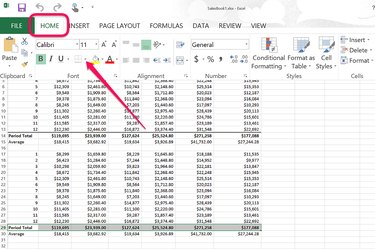
Highlight the cells in your Excel worksheet that you want to have a border, or cells that have a border with a color you want to change. Click the "Home" menu, then click the "Border" icon in the Fonts group. Another way to reveal the Border menu is to right-click the highlighted cells and select "Format Cells."
Step 2
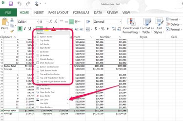
Select any Border Style from the Border drop-down menu, then click the "Line Color" option. If you want the border color to be easily noticeable, select a thick border style.
Step 3
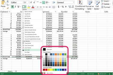
Select any color from the palette to use for the border. For a wider selection of colors, click the "More Colors" link. After selecting a color, click anywhere on the worksheet to see how your border looks around the cells you highlighted.