How to Compare Cells in Excel

Conditional Formatting also helps workbooks look nicer.

Image Credit: Image courtesy of Microsoft

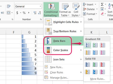
In Excel 2013, the IF function serves to compare cells regardless of their position. In many cases, however, you don't need to go through the hassle of writing a formula just to check how cells compare. To search for duplicates, to find cells above an average value or to style cells based on their values, use Conditional Formatting as the fastest way to compare cells.

Conditional Formatting

Video of the Day

Step 1

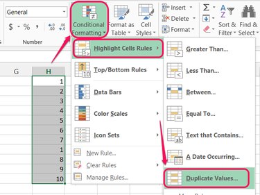
Other Highlight Cells Rules check for Greater Than or Less Than conditions.

Image Credit: Image courtesy of Microsoft

Select a range of cells to compare internally, open the Conditional Formatting menu on the Home tab, point to Highlight Cells Rules and choose Duplicate Values. This feature works well to track down accidental duplicates or find matching items in a long list, but it doesn't work across multiple sheets.

Video of the Day

Step 2

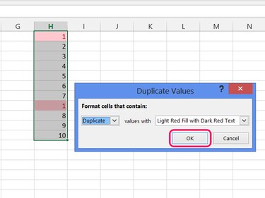
The other option in the first menu highlights unique values.

Image Credit: Image courtesy of Microsoft

Leave the first drop-down menu set to Duplicate, change the coloring option if you want and press OK to highlight duplicate cells.

Step 3

Clearing formatting does not affect cell values.

Image Credit: Image courtesy of Microsoft

Delete a duplicate cell to remove the highlighting from its partner.

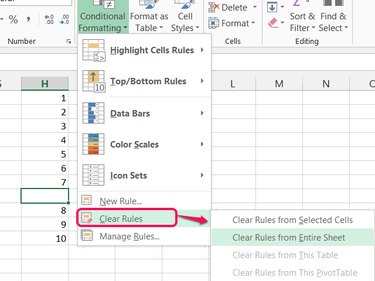
If a duplicate value occurs again later, Excel automatically highlights the cells again. To turn off highlighting permanently, reopen Conditional Formatting and choose one of the options from the Clear Rules menu.

Step 4

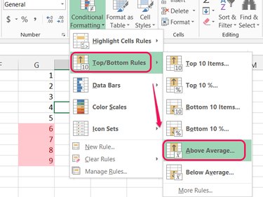
Click New Rule to write a custom rule using a formula.

Image Credit: Image courtesy of Microsoft

Use other conditional formatting options to compare cells in other ways. For example, the Above Average option listed under Top/Bottom Rules highlights cells above the average for the selected range.

Step 5

Excel can display multiple conditional formats at the same time.

Image Credit: Image courtesy of Microsoft

Add Data Bars or Color Scales from the Conditional Formatting menu to help visualize the relative difference between cell values.

Compare Cells Using Formulas

Step 1

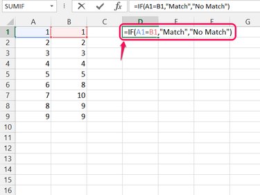
Cells don't need to be adjacent to compare them.

Image Credit: Image courtesy of Microsoft

Check whether two specific cells match using the IF function. Start a formula with =IF( and enter the two cell locations, separated by an equal sign. Add a comma and enter the text, in quotes, to display if the cells match. Add another comma and then the text, in quotes, for a non-match.

For example, the formula could read =IF(A1=B1,"Match","No Match") to compare cells A1 and B1. Press Enter to finish the formula.

Step 2

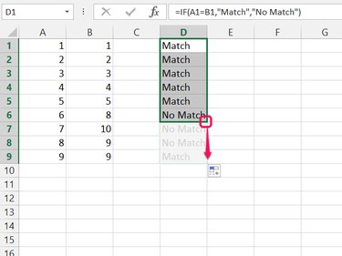
Or double-click the corner to auto-fill to the bottom of the adjacent column.

Image Credit: Image courtesy of Microsoft

Drag the lower-right corner of the formula's cell to extend it to other cells and compare two columns or rows.

Step 3

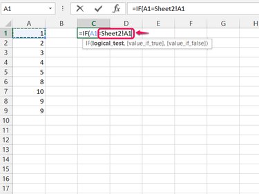
This also works between workbooks with the notation [Book]Sheet!Cell

Image Credit: Image courtesy of Microsoft

Use the notation Sheet!Cell to refer to cells on other spreadsheets while building the formula. For example, Sheet1!A1 to reference cell A1 on Sheet1. You can also switch to another sheet and click a cell in the middle of typing a formula to insert the cell's location.

Step 4

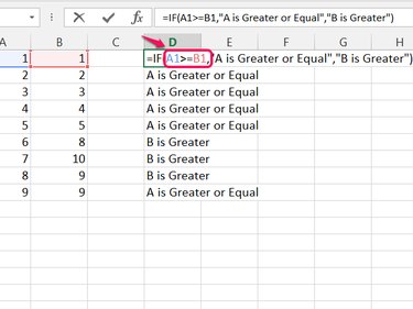
The results update automatically when the referenced cells change.

Image Credit: Image courtesy of Microsoft

Substitute the greater-than or less-than sign for the equal sign to compare cells for conditions other than exact matches. Use >= or <= to check for greater-than-or-equals or less-than-or-equals conditions, respectively.